Texas Flood: Modeling the Colorado River in Texas
|
|
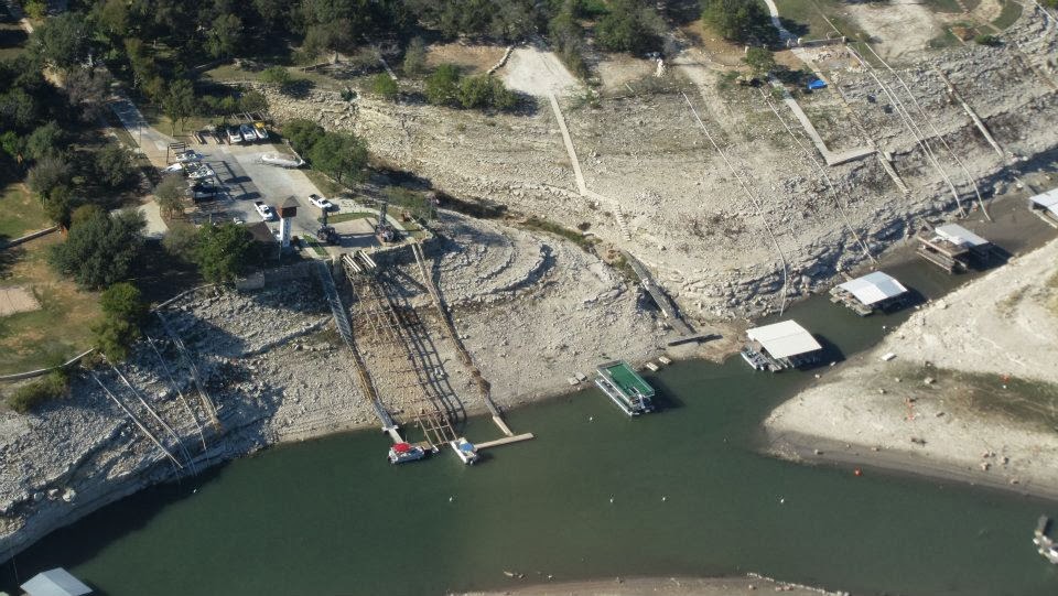 |
| Lake Travis shoreline down 52 feet |
Lake Travis is a manmade lake, fed by the Colorado River (not the one that runs through the Grand Canyon, this one). In addition to being a great place to spend a hot Texas summer day, Lake Travis provides all the drinking and irrigation water for the city of Austin and much of central Texas. So when lake levels get low, people start getting nervous.
It's been a while since I've seen the lake full, so I started wondering what it would take to fill the lake up to normal levels. Obviously it's not just a matter of getting rain, we need rain to fall in the watershed of Lake Travis in order to capture it. This is why, despite the wetter than average Fall and Winter we've had in Austin, Lake Travis hasn't seen a significant rise in water level. All that rain is falling downstream of the lake, and (unfortunately) flowing out to the Gulf of Mexico uncaptured.
To better study the lake, and the Colorado River that feeds it, I went in search of historical data I could use to train a model of the Colorado River. What I found was probably overkill for the job: historical lake elevations in 15-minute intervals, flow rates from USGS gauges in every stream and river in the American Southwest (also in 15-minute intervals), and daily rainfall totals from NOAA across much of Texas. I then set about cleaning up the data to get it into a more manageable format. Focusing only on a period from January 1, 2011 to December 31, 2012, I calculated daily averages for Lake Travis and trimmed the weather data to include only stations located in the Colorado River basin. The real pain came from the USGS stream flows data.
The file containing the data had about 30 million records, and was over 1 GB in size. While this is kind of big, it's not prohibitively so. I probably could have written something to scan the file sequentially and ran in on my laptop without too much trouble, but I wanted to try something clever. I've written about Pig--the Hadoop-based programming tool that lets you easily parallelize map-reduce-style jobs--before, and I have been looking for a project that's big enough to use it again. Pig is one of the tools used by real data scientists to analyze very large datasets (think TB and even PB), so I set out to use it to clean up my meager 1 GB file. I spun up a cluster of 10 machines running Hadoop using Amazon Web Services and ran the Pig script I developed. The script selects only those sites located in the Colorado River basin, and computes a daily average from their 15-minute interval measurements. The great thing about Pig is that if I somehow found myself with 1,000 times more data in the future, I could re-run the script again without changing a thing; I'd only need to request more CPU time.
With my data cleaned and scrubbed, I was ready to re-cast my problem into the language of machine learning. What I had were training data, and I wanted to train a model on the Colorado River basin in order to predict the outcome of future rainfall on the lake levels. This post will deal with the model training, and in a future one I'll show what would happen if central Texas was hit by a major tropical storm--a scenario many people claim we need if we want to get Lake Travis back to full.
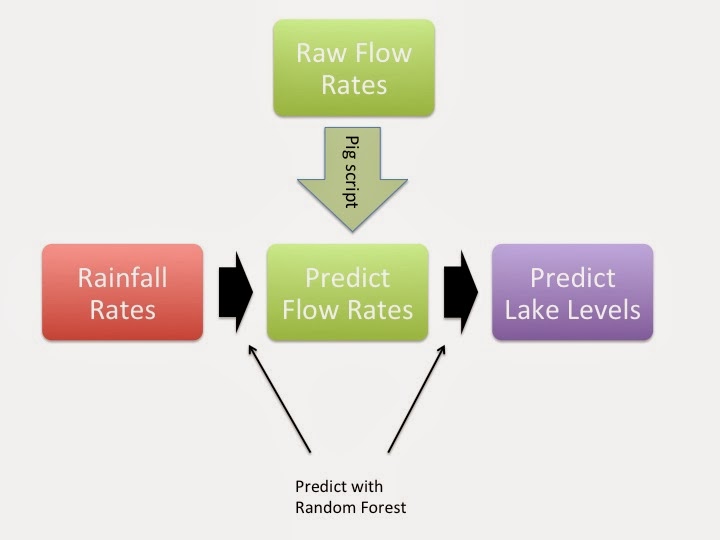 |
| A flowchart describing my model of Lake Travis and the Colorado River |
In the parlance of machine learning, "features" are equivalent to dependent variables--in my case these are the different stations recording rainfall or stream flows. The term "examples" refers to the number of different observations--in my case this would be each day's observations. The challenge of the model is then to learn a way to map the training set's features to the observations. So I arranged my training data in the standard way:
I treated each day's observations as an example, with the idea that I would train the model and then feed it new flow rates (which I would simulate from a tropical storm) and calculate Lake Travis's elevation that day. However, it immediately became obvious that there needed to be a time delay. The Colorado River is over 800 miles long so it will take water an unknown length of time to propagate down the river. Flow rates of streams near its source in New Mexico will not be reflected in Lake Travis's elevation for the same day. So I added a time delay to the matrix X:
 |
Here I added the flow rate for each station up to p days earlier as additional features. |
Each station's daily value would still be a feature, but I also added the station's values during the previous p days. Even if different parts of the river experience different delays, the model will be able to pick the appropriate feature to fit to (i.e. it will find the right delay for each station). In my final model, I set p to 5. Of course, I tested to ensure the results don't depend on p--the maximum delay built in.
Now I was finally ready to run the models. I used the randomForestRegressor model from the scikits-learn package in Python. A random forest is collection of decision trees that attempt to fit the data by developing rules for how the training examples map to observations of the target values. There are very sophisticated algorithms for creating the set of rules that performs the mapping. I won't go into detail here, but random forests create many decision trees using bootstrap-resampled data and then use a majority vote amongst the trees to determine the optimal set of rules for the mapping.
Here's my program that implements this modeling procedure. I ran it and found I was able to predict the lake's level pretty accurately from the stream flow data alone:
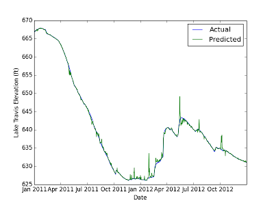 |
| Source Code My model is able to fairly accurately predict the elevation of Lake Travis from historical data of the Colorado River and its tributaries. I'm a bit concerned about those spikes where the model sometimes disagrees by 5 feet or so for a short time period, but I'll worry more about that when I'm trying to predict future levels. |
This means I have an accurate model of the Colorado River basin. However, a good model also needs to be able to generalize well to fit new examples it hasn't seen before (called the test set). This will become very important in the future when I want to predict future lake levels from a hypothetical storm. However, for the moment I'm not as concerned about overfitting since I'm really only focusing on the training data. For now, I really just want to know where rain needs to fall to get into the lake. As I'll show, the model makes intuitive sense to me so for now I'll trust it isn't overly complex.
So now let's try to answer the question of which streams influence the lake level most significantly. A great side benefit of using random forest models is that they also give some information about the relative importance of each feature to the fit of the model:
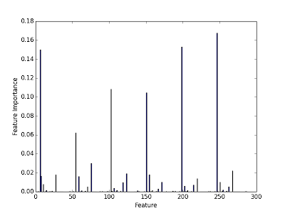 |
Source Code Here are the importances of each stream in the determination of Lake Travis's elevation. Clearly there are a few cases that are very important in determining the final prediction. |
I can select the top k most important features and examine them. This tells me about the streams (with their built-in time delays) that most significantly impact the water level in Lake Travis.
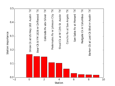 |
Source Code The top 10 most important features (stream gauges) in determining Lake Travis's elevation. |
I can put these stations on a map of the basin and show the locations of the important streams and minor rivers that have the most impact on the level of Lake Travis. When it rains near these streams, the lake rises significantly in the following 1-10 days.
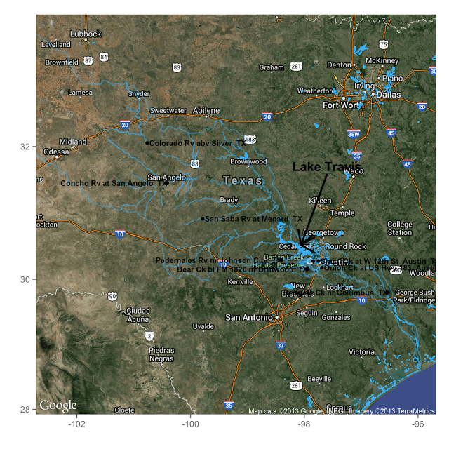 |
| Source Code Map of the rivers and streams that most significantly influence water levels in Lake Travis. |
Looking at the map, I feel pretty good about the model. I've heard weathermen say that we need rain in the Hill Country west of Austin so that the Pedernales River will fill up and bring water into Lake Travis. Likewise, the San Saba River and Concho River are also major known tributaries to the Colorado. However, there is one puzzling fact that stands out: 5/9 of the stations plotted are downstream of the lake! Clearly high flow rates in these streams can't cause Lake Travis to rise. I think this is a classic correlation vs. causation issue. I was interpreting the important features, according to my random forest model, as causal. This is not necessarily true, and the feature importance algorithm will really only pick out features that correlate strongly with changes to the target observable. However, intuition suggests that the streams found to be important, that are upstream of the lake, should probably influence Lake Travis in a causal way. After all, water flows downhill.
So the takeaway is that it probably needs to rain near Johnson City, Menard, San Saba, and Silver for water to get into the lake. Stay tuned to future posts, where I'll try to use the other part of the modeling to predict stream flow rates and future lake levels from a simulated tropical storm over central Texas.

Leave a Comment